HALLOWED TURF
Computer Vision
This page has all the projects that I have implemented so far, as part of the coursework for the Computer Vision course under the Robotics Institute at CMU. I was inspired the huge potential of Computer Vision in Augmented Reality while working in the Mixed Reality (MREAL) solutions team as an intern at Canon Inc. Hence I have taken this course which introduces me to the fundamental techniques used in computer vision, that is, the analysis of patterns in visual images to reconstruct and understand the objects and scenes that generated them. All the projects were implemented in MatLab.
Spatial Pyramid matching for Scene Classification
This project consisted of two phases:
1) Visual representation of images by a using a 'Bag-of-Words':
We apply a set of 20 filters on every training image and create a visual representation for each image based on it's filter response. Then we use K-means clustering on the filter responses to create a dictionary of visual words.


Building a recognition system:
1) Count the number of times a visual word appears in an image.
2) Use spatial pyramid matching to get spatial information of the scene. That is we find out how many times each word appears in each section of the image.
3) Now we use nearest neighbor technique to compare each test image with the training image set and then deduce the label of the scene.
For example for the image used above will be classified as an airport. Below is a screen shot of the MATLAB command window:

BRIEF feature descriptor and matching
In this project, given an image, we have to find the key feature points (Keypoints), generate descriptors for each of those keypoints and then match them with those of another image.
Keypoint detection:
Keypoints in an image are points which can be used to distinctly identify an object. These maybe be blobs, corners or high intensity pixels. So the following steps were done to a set of keypoints for an image:
1) Created a Gaussian Pyramid of 5 levels.
2) A Difference of Gaussian (DoG) pyramid was created from the above.
3) Principal curvature ratio (a higher ratio would mean there is a curvature across an edge) was found for each level. This would help us suppress keypoints which are on the edges as these keypoints are not distinct and are difficult to localize.
4) Local Extremas within a neighborhood of 10 pixels (8 surrounding pixels in the same space and one above and below in the scale space) were detected. Thresholds for DoG response and principal curvature were also enforced.
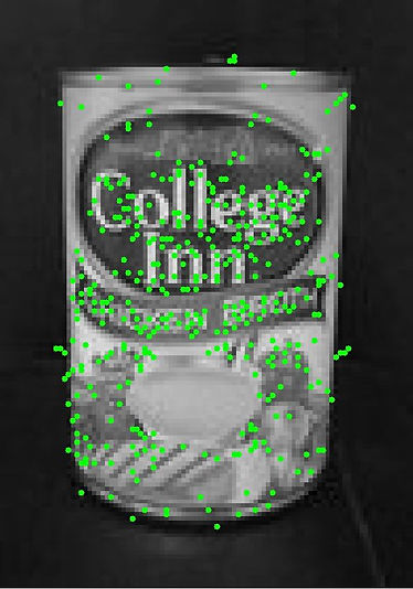
Below are the keypoints generated for an image of a chicken broth can:

BRIEF descriptors and matching:
BRIEF stands for Binary Robust Independent Elementary Features. It is one of the methods of describing a region around an image. It is a binary descriptor as it compares the intensity levels of a pair of pixels and returns 1 if one is less than the other and 0 otherwise. We chose 256 pairs of pixels in a 9 x 9 neighborhood around each keypoint. We then compare descriptors of two images and store all the matches between them.
The following shows the matches made between two images.

Homography and Panorama
In this assignment, I understood what the Homography matrix is used for and how it can be estimated given corresponding feature points in the two images taken from two different camera points. In the first part I estimated the Homography matrix H given two sets of corresponding feature points p1 and p2. I then normalized the homography matrices using a transformation matrix having a scale factor and translation. The homography matrix was then used to create a panoramic image from two given images of the Taj Mahal, as shown below:
Given images of the Taj taken from two viewpoints:


Panoramic image created using the H matrix.

In the next step, I created a mosaic view of the images in which all the pixels in the panoramic image obtained earlier are visible. i.e The I created a estimated a frame using the homography matrix and the edges of the warped image. Finally I displayed the panoramic image within the frame as show below:

Lucas-Kanade Optical-Flow
In this assignment, I have tracked a car in a given video sequence using Lucas-Kanade template tracking. Lucas-Kanade template tracking basically assumes that the template undergoes constant motion in a small region. The algorithm estimates the deformations between two image frames given a particular starting template. In the assignment, the rectangular coordinates of the car in the first frame is given to us and Lucas-Kanade is performed for every two consecutive frames. Here is the resulting video of the same. NOTE: The original clip is 3 seconds long and the frame rate is reduced in order to increase the duration of the final video.
In the second part of the assignment I implemented Lucas-Kanade tracking using appearance basis. So I was given a set of template images of the object to be tracked, taken under various illumination conditions. I used these basis vectors and implemented a gradient descent to simultaneously minimize the change between two consecutive frames. The below video demonstrates that the object is being tracked fairly accurately despite moving from dark to bright illumination.